Show Negative numbers in Red color in Google Sheets document
There are two different ways to highlight negative numbers in red color in a Google Sheets document. These are: Let’s check both the options one by one.
1] Highlight negative numbers in red color in a Google Sheets document using Conditional Formatting
The conditional formatting option highlights the entire cell with red color that has negative numbers. You can also choose a custom color of your choice to highlight negative numbers. Let’s check the steps: That’s it. Now you will notice that all the negative value cells selected by you are highlighted with the red color or the color chosen by you. As you change the values in the selected cells, the color will be changed accordingly because of the rule set by you. Also read: How to change Date format in Google Sheets and Excel online.
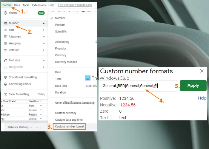
2] Show negative numbers in red color in a Google Sheets document using Custom Formatting
Using custom formatting, the color of selected cells is not changed, only the value color present in the selected cells is changed in red color. You can’t set a custom color to highlight negative numbers, only red color is there. Here are the steps: This will immediately highlight negative values with red color in the cells selected by you. Whenever you will change the values in the cells where you have applied the custom formatting, the color for negative values in those cells will change automatically.
How do you highlight negative numbers in red?
If you want to highlight the negative numbers in red in a Google Sheets document, then there are two ways for doing this. You can use the conditional formatting and custom formatting options present under the Format menu of your Google Sheets document. While the first option lets you fill or highlight the selected cells (having negative numbers) with red color or a custom color, the latter option lets you highlight negative values in selected cells with red color only. We have already covered both the options separately with a step-by-step guide in this post above.
How do I color numbers in Google Sheets?
You can use the conditional formatting option available under the Format menu of a Google Sheets document to highlight or color cells for the numbers or values. For example, you can set a rule that if the value present in the selected cell(s) is greater than 10, then that cell will be filled or highlighted with the green color or some other color of your choice. Hope it is helpful for you. Read next: How to add an image in Google Sheets.